
Advanced Shadow Mapping
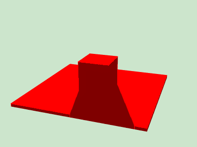
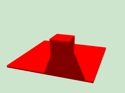
The previous post introduces the basics of shadow mapping. However, I didn’t mention one of the fundamental problems: aliasing. If we take a closer look at the shadow, we will find it jagged on the edge.
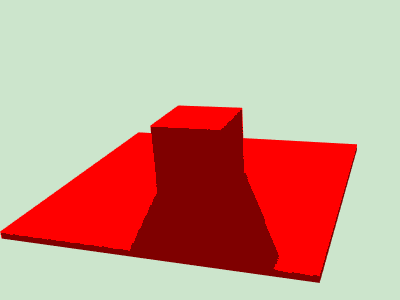
This is a common problem for pre-computed texels: if we had a depth map of infinite resolution, the problem would have been solved. The shadow acne problem is also caused by this, though it could be hidden by applying a small bias. However, we have no luck for aliasing.
A lot of research has been done to mitigate aliasing, and to create soft shadow at the edge to look more realistic, such as Percentage Closer Filtering, Variance Shadow Maps, Moment Shadow Mapping.
Percentage Closer Filtering
This is one of the most fundamental work. For simplicity, I’m only going to walk through a very basic version of it. The idea is intuitive: instead of sampling from a texel that is closest to the true coordinate, sample from a window (e.g. 2x2), and do an average (or weighted average, according to distance).
Remember the way we sample from the depth texture
texture(uDepth, lightCoord.xy);
Instead of doing this, we sample from a window of texels. For clarity, let’s say uDepthMapScale is passed in as uniform that is equal to vec2(1./depthMapWidth, 1./depthMapHeight). Also we enlarge the window a little bit (4x4) to get fuzzier edges.
float x, y, visibility = 0.;
for (y = -1.5; y <= 1.5; y += 1.) {
  for (x = -1.5; x <= 1.5; x += 1.) {
    float occluderLightDist =
        texture(uDepthMap, lightCoord.xy + uDepthMapScale * vec2(x, y)).z;
    visibility += weight(x, y) * float(fragLightDist < occluderLightDist + kEps);
  }
}
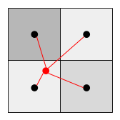
More formally, let’s define $z_f$ as the distance from fragment to light and $z_o$ as the distance from occluder to light. Given a depth window in the view of light, the window of $z_o$’s, let’s say $Z_o$, the visibility of the fragment could be modeled as
where $W$ is the filter, $*$ is convolution, and $I$ is indicator function. For example, if we apply a 2x2 average filter on a depth window like this
then $V(z_f)$ would be a multi-step function
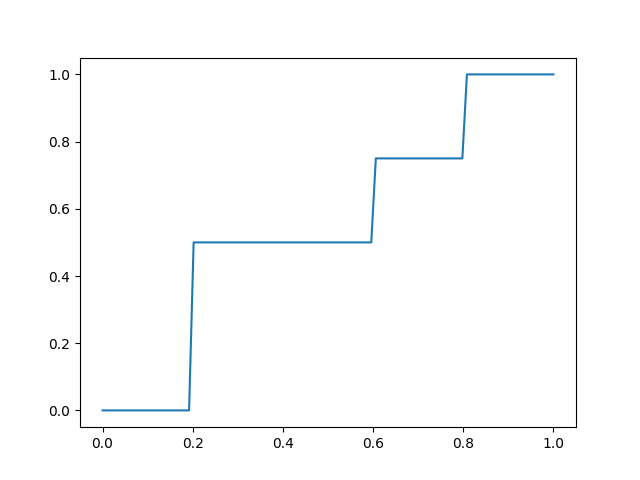
For $z_f$ that is on the edge of a step, there still might be chance of shadow acne or aliasing.
Variance Shadow Maps
Given a pre-computed depth map and a texture coordinate $(x, y)$, the $z_o$ sampled from it is actually an inaccurate one: some information has already been lost due to the finite rasterization. The true $z_o$ is actually a random variable that we don’t know; the convolution we did in PCF is neverthless a good guess based on the continuity nature of the real scene.
However, in PCF we have to apply a convolution kernel per fragment in the shadow pass, which could be expensive if the kernel size is very large. Then someone asks the question: can we pre-compute the convolution in the depth pass, and only sample from one texel in the shadow pass? One of the benefits is that, if the light doesn’t move, in other words, the pre-computed depth map doesn’t change, the shadow pass could be much rendered much faster.
Actually, to sample $z_o$ from a window, we don’t need all the values from it; some statistics about the window might be good enough. In Variance Shadow Maps, the author proposes to collect the first two moments per window in the depth pass, and model the visibility as
The inequality is Chebychev’s inequality. $\mu$ and $\sigma$ could be pre-computed in the depth pass.
$z_o$’s are sampled per window, so they could be pre-computed via convolution. For clarity, let’s say the pre-computed result will have each texel being the weighted average of $(z, z^2, 0, 1)$ of a window around it. Given a texel sample, and the fragment-light distance, we can compute the visibility as following
float computeVisibility(vec4 depthMapSample, float fragLightDist) {
  float mu = depthMapSample.x;
  if (mu > fragLightDist) {
    return 1.;
  }
  float mu2 = mu * mu;
  float sigma2 = clamp(depthMapSample.y - mu2, 1e-8, 1e8);
  float fragOccluderDist = fragLightDist - mu;
  float fragOccluderDist2 = fragOccluderDist * fragOccluderDist;
  return sigma2 / (sigma2 + fragOccluderDist2);
}
Notice that we applied a trick by early return at mu > fragLightDist. Otherwise, there will be very bad artifact at fragment where $z_f < z_o$ for real.

From math, we can easily analyze the side effect of the term $(z_f - \mu)^2$, so to avoid the risk, we simply ignore this term when $z_f < \mu$.
This method is not perfect neither. Notice that we modeled the visibility as upper bound of $P(z_o \ge z_f)$. The upper bound may not be tight, so there’s chance that the visibility is greater than its true value. The consequence is that some region will be brighter than what it should be, and this artifact is known as Light Bleeding.
Moment Shadow Maps
Is it possible to get a closer upper bound given more moments? The answer is yes. In Moment Shadow Maps, the author generalizes the problem as Hamburger Moment Problem, and gives the following solution with 4 moments.
- Let $b = (z, z^2, z^3, z^4)$
- Let $b’ = (1 - \alpha) \cdot b + \alpha \cdot (0., .63, 0., .63)^T$, $\alpha = 9 \cdot 10^{-3}$
- Solve $c$ with Cholesky decomposition
- Solve $d_1 \le d_2$ for
- Compute visibility given $z_f$, $b’$, $d$.
float computeVisibility(vec4 depthMapSample, float fragLightDist) {
  float alpha = 9e-3;
  vec4 b = (1. - alpha) * depthMapSample + alpha * vec4(0., .63, 0, .63);
  mat3 B = mat3(
      1.0, b.x, b.y,
      b.x, b.y, b.z,
      b.y, b.z, b.w);
  float zf = fragLightDist;
  vec3 z = vec3(1, zf, zf * zf);
  vec3 c = inverse(B) * z;
  float sqrtDelta = sqrt(c.y * c.y - 4. * c.z * c.x);
  float d1 = (-c.y - sqrtDelta) / (2. * c.z);
  float d2 = (-c.y + sqrtDelta) / (2. * c.z);
  if (d2 < d1) {
    float tmp = d1; d1 = d2; d2 = tmp;
  }
  if (zf <= d1) {
    return 1.;
  } else if (zf <= d2) {
    return 1. - (zf * d2 - b.x * (zf + d2) + b.y) / ((d2 - d1) * (zf - d1));
  } else {
    return (d1 * d2 - b.x * (d1 + d2) + b.y) / ((zf - d1) * (zf - d2));
  }
}
Quantization
TODO